Introduction to Measures of Spread
Watch this topic in 60 seconds
Free preview · Lesson 1
Understanding Introduction to Measures of Spread
Introduction to Measures of Spread: Beyond the Average!
Imagine you're trying to understand a group of numbers. Maybe it's the test scores of a class, the daily temperatures in a city, or the salaries of employees in a company. Often, the first thing we look at is the 'average' (or mean, median, mode) to get a general idea. These are called Measures of Center, and they tell us where the 'middle' or 'typical' value of our data lies.
But here's a secret: knowing the average isn't always enough to truly understand what's going on! Think of it this way:
Analogy: The Ice Cream Shop Mystery
You have two ice cream shops, 'Creamy Dream' and 'Sweet Spot'. Both claim their average waiting time for customers is 5 minutes. Sounds great, right? But what if at Creamy Dream, sometimes you wait 1 minute, sometimes 3, sometimes 7, and sometimes 9? It's always around 5 minutes, but the wait times can swing quite a bit. At Sweet Spot, you almost always wait 4, 5, or 6 minutes – very consistently around 5. Both have the same average, but your experience could be very different! Creamy Dream has more spread in its wait times.
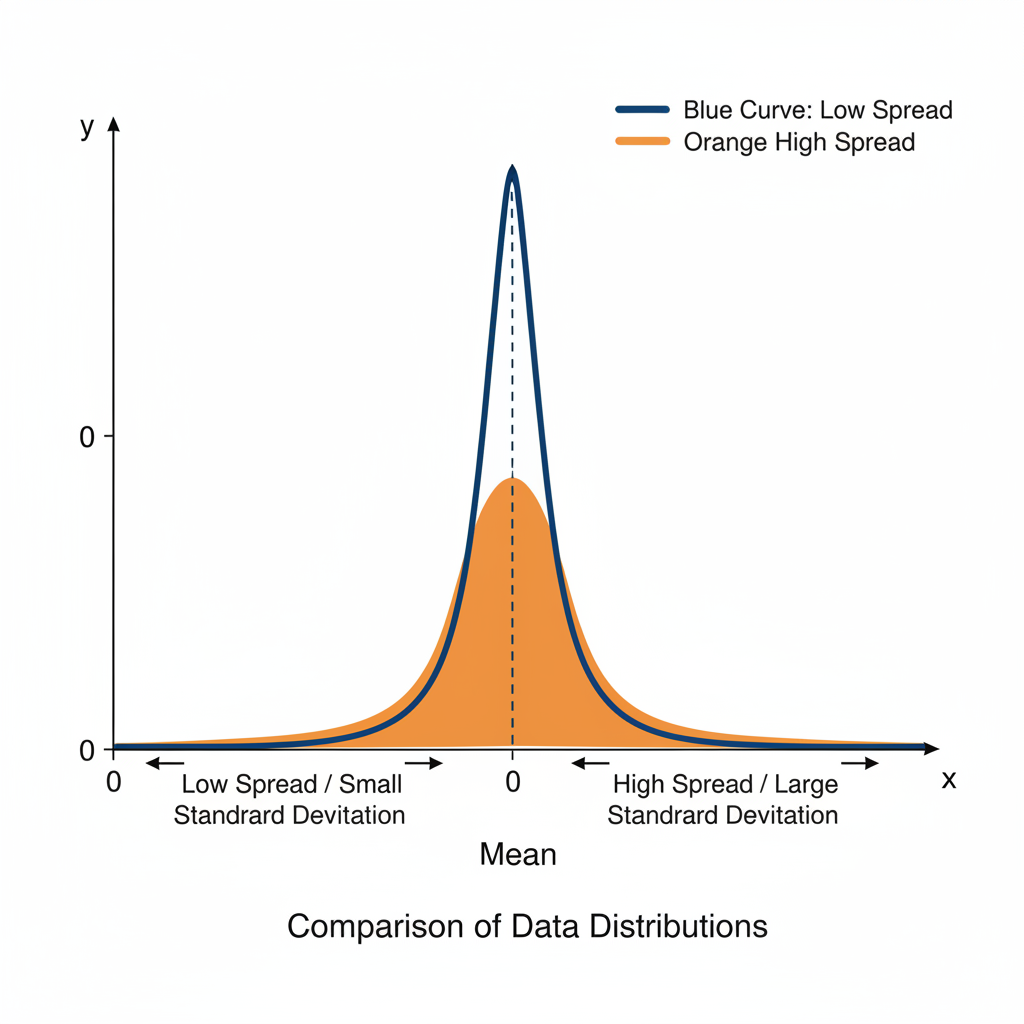
This is where Measures of Spread (also known as Measures of Variability or Dispersion) come in. They tell us how 'stretched out' or 'bunched up' our data is. They answer questions like: How consistent are the numbers? How much do they vary from each other? Are all the values close to the average, or are some very far away?
Why Are Measures of Spread So Important?
Measures of spread help us make better decisions and understand the full picture. Here are a few reasons:
- Understanding Consistency: Is a student consistently scoring around 80%, or do they swing wildly between 50% and 100%?
- Comparing Groups: If two classes have the same average test score, the one with less spread might be more consistently performing, perhaps indicating a more stable learning environment.
- Risk Assessment: In finance, two investments might have the same average return, but the one with less spread (less variability) is generally considered less risky because its returns are more predictable.
- Quality Control: A factory wants its products to be consistently the same size. Low spread in measurements means high quality control.
Core Concepts of Spread: Unpacking the Data
1. The Range: The Simplest Picture of Spread
The range is the most basic way to understand how spread out a set of numbers is. It's super easy to calculate!
Analogy: The Height Difference
Imagine you're in a room with 10 people. The shortest person is 150 cm tall, and the tallest is 190 cm tall. The range of heights in that room is 190 cm - 150 cm = 40 cm. This tells you the total span from the absolute lowest to the absolute highest value.
Definition: The Range is the difference between the highest (maximum) value and the lowest (minimum) value in a dataset.
Formula: Range = Maximum Value - Minimum Value
Example: Test scores: 60, 75, 80, 85, 90 Maximum = 90, Minimum = 60 Range = 90 - 60 = 30
Strengths:
- Very easy to understand and calculate.
- Gives a quick idea of the total span of data.
Weaknesses:
- Highly affected by outliers: If one student scored a 10 and everyone else scored above 70, that single low score would drastically increase the range, even though most scores are close together. It only uses two pieces of information (the max and min), ignoring everything in between.
2. The Interquartile Range (IQR): Focusing on the Middle Ground
Because the range can be so easily skewed by extreme values, mathematicians developed a more robust measure of spread: the Interquartile Range (IQR).
Analogy: The Movie Critics' Consensus
Imagine 100 movie critics review a film. If you only look at the highest score and the lowest score (the range), two critics who loved it and two who hated it could make the movie seem very controversial, even if 96 critics gave it average scores. The IQR is like ignoring the most extreme 25% of positive and negative reviews and focusing only on the scores of the middle 50% of critics. This gives a more stable picture of how the movie was generally received.
The IQR focuses on the spread of the 'middle 50%' of your data. To understand it, we first need to understand quartiles.
What are Quartiles?
Just like the median divides your data into two equal halves (50/50), quartiles divide your data into four equal parts (25% each).
- Q1 (First Quartile): This is the median of the lower half of your data. 25% of the data falls below Q1.
- Q2 (Second Quartile): This is the overall median of your entire dataset. 50% of the data falls below Q2.
- Q3 (Third Quartile): This is the median of the upper half of your data. 75% of the data falls below Q3.
Definition: The Interquartile Range (IQR) is the difference between the third quartile (Q3) and the first quartile (Q1).
Formula: IQR = Q3 - Q1
How to Calculate IQR:
- Order the Data: Arrange all your numbers from smallest to largest.
- Find the Median (Q2): This splits the data into a lower half and an upper half. (If there's an even number of data points, the median is the average of the two middle numbers; the median itself is usually NOT included in the halves when calculating Q1 and Q3 for an odd number of data points).
- Find Q1: Find the median of the lower half of the data.
- Find Q3: Find the median of the upper half of the data.
- Calculate IQR: Subtract Q1 from Q3.
Example: Test scores: 60, 65, 70, 75, 80, 85, 90, 95, 100 (9 data points)
- Ordered data: 60, 65, 70, 75, 80, 85, 90, 95, 100
- Median (Q2): 80 (the middle value)
- Lower half: 60, 65, 70, 75. Q1 = Median of lower half = (65+70)/2 = 67.5
- Upper half: 85, 90, 95, 100. Q3 = Median of upper half = (90+95)/2 = 92.5
- IQR = Q3 - Q1 = 92.5 - 67.5 = 25
Strengths:
- Robust to Outliers: Since it ignores the lowest 25% and highest 25% of data, extreme values don't affect it as much as they do the range.
- Gives a clearer picture of the spread for the majority of the data.
Weaknesses:
- Ignores the extreme values completely (the very lowest and very highest data points).
- Slightly more complex to calculate than the range.
3. Variance and Standard Deviation: The 'Average Distance' from the Mean (Conceptual)
While Range and IQR are great for a quick look, statisticians often use Variance and Standard Deviation because they consider every single data point and how far it is from the mean. For 10th grade, we'll focus on understanding what they represent rather than getting deep into their calculation formulas, which can be quite complex without a calculator or software.
Analogy: How Far is Everyone from the Team Captain?
Imagine a soccer team standing in a line, and the captain is in the middle. The Range would be the distance from the person furthest left to the person furthest right. The IQR would be the distance between the person at 25% mark and the person at the 75% mark. But Variance and Standard Deviation are like calculating, on average, how far each player is from the captain. If everyone is huddled close to the captain, the 'average distance' is small (low spread). If players are scattered all over the field, the 'average distance' is large (high spread).
Variance: This measures how far, on average, each number in the dataset is from the mean. It specifically measures the average of the squared differences from the mean. Squaring the differences ensures that negative differences don't cancel out positive ones, and it emphasizes larger differences.
Standard Deviation: This is simply the square root of the Variance. Taking the square root brings the units back to the original unit of measurement, which makes it much easier to interpret than variance. If your data is in kilograms, the variance would be in 'kilograms squared', which doesn't make much sense. Standard deviation would be back in 'kilograms'.
Key Idea:
- A small standard deviation means the data points are generally close to the mean (low spread, high consistency).
- A large standard deviation means the data points are generally spread out over a wider range of values (high spread, low consistency).
Strengths:
- Uses every data point in its calculation, providing a more comprehensive measure of spread.
- Crucial for more advanced statistical analysis.
- Standard deviation is in the same units as the original data, making it interpretable.
Weaknesses:
- More complex to calculate manually.
- Sensitive to outliers (like the mean, which it relies on).
Putting it All Together: Why We Need Both!
Understanding measures of center (like mean and median) alongside measures of spread (like range, IQR, and standard deviation) gives us a much more complete and accurate picture of any dataset. The mean tells us 'where' the data tends to be, and the standard deviation tells us 'how consistently' it's there. The median tells us the true middle, and the IQR tells us how spread out the middle part is.
Remember: Numbers alone don't tell the whole story. Context and a variety of statistical tools help us truly understand the world around us!
As you move forward in statistics, you'll find that different measures of spread are useful in different situations, depending on the type of data you have and what questions you're trying to answer. For now, grasp the core idea that spread matters just as much as the average!
Keep learning, free
Create a free Syllabax account to unlock practice questions and games for this topic.
Visual Learning Enhanced! 🚀
To help you master this topic, we use Advanced Syllabax AI to generate detailed diagrams and visual models.
Note on Visuals: The AI sometimes makes spelling errors in image labels. Please refer to the lesson text for the correct terminology.