Ogive (intro) (Statistics)
Watch this topic in 60 seconds
Free preview · Lesson 1
Understanding Ogive (intro) (Statistics)
Understanding Ogives: A Cumulative Journey Through Data (Grade 10 Foundations)
Welcome, future data detectives! Today, we're going to uncover a fascinating tool in statistics called an Ogive (pronounced OH-jive). Don't let the fancy name scare you; it's simply a special kind of graph that helps us see data in a very useful way: cumulatively. Think of it like a journey where you're always adding up what you've collected along the way.
What is an Ogive? The Running Total of Your Data!
Imagine you're tracking how many steps you take each day. A regular bar graph (histogram) might show you the steps for Monday, then Tuesday, then Wednesday. But what if you wanted to know your total steps accumulated by Wednesday? That's where cumulative thinking comes in! An Ogive is a smooth curve graph that shows us the cumulative frequency of a dataset.
Analogy 1: Building a Lego Tower. Each brick you add represents a 'frequency' – how many times something happened in a specific category. A regular bar graph shows the height of each individual brick. But an Ogive is like looking at the *total height* of your tower after adding each new section. It's always growing upwards, showing you the running total.
Before We Dive In: Key Ingredients
To understand Ogives, we need to quickly review a few core concepts:
- Frequency Distribution: This is just a table that shows how often each value or group of values (called 'class intervals') appears in your data. For example, how many students scored between 0-20 marks, 21-40 marks, etc.
- Class Intervals: These are the groups or ranges into which we sort our data. Like 0-10, 11-20, 21-30, and so on.
- Class Limits: For each class interval, there's a lower limit (the smallest value) and an upper limit (the largest value). For 0-10, 0 is the lower limit and 10 is the upper limit.
The Heart of the Ogive: Cumulative Frequency
This is the most crucial concept. Cumulative frequency is simply the running total of frequencies. You start with the frequency of the first class, then add the frequency of the second class to it, then add the frequency of the third class to that sum, and so on.
Analogy 2: Filling Buckets. Imagine you have several buckets, and each bucket represents a class interval (e.g., students who scored 0-20, 21-40, 41-60). The amount of water in each individual bucket is its 'frequency'. Now, imagine you pour all the water from the first bucket into a large tub. Then you pour the water from the second bucket into the *same tub*, adding to what's already there. Then the third bucket, and so on. The amount of water in the large tub at any point is your 'cumulative frequency' – the total amount accumulated so far.
Let's Construct an Ogive: The 'Less Than' Type
There are two main types of Ogives: 'Less Than' and 'More Than'. For a foundational understanding, we'll focus on the 'Less Than' Ogive, which is the most common and intuitive.
A 'Less Than' Ogive tells us how many observations are less than a certain value. For example, how many students scored less than 70 marks?
Steps to Create a 'Less Than' Ogive:
-
Prepare Your Frequency Distribution Table: Start with your raw data and organize it into class intervals with their corresponding frequencies.
Marks (Class Interval) Number of Students (Frequency) 0-20 5 21-40 12 41-60 18 61-80 10 81-100 5 -
Calculate 'Less Than' Cumulative Frequency: Add a new column to your table for 'Upper Class Limit' and 'Cumulative Frequency'. For a 'Less Than' Ogive, we plot the cumulative frequencies against the upper class limits of the class intervals.
Marks (Class Interval) Number of Students (Frequency) Upper Class Limit Cumulative Frequency (CF) 0-20 5 20 5 (students scoring less than 20) 21-40 12 40 5 + 12 = 17 (students scoring less than 40) 41-60 18 60 17 + 18 = 35 (students scoring less than 60) 61-80 10 80 35 + 10 = 45 (students scoring less than 80) 81-100 5 100 45 + 5 = 50 (students scoring less than 100) -
Choose Your Axes:
- X-axis (Horizontal): Mark the Upper Class Limits (or class boundaries if data is continuous). Make sure to start with a point representing a cumulative frequency of 0, corresponding to the lower limit of the first class interval (or slightly before). For our example, you might start with 0 on the x-axis for a CF of 0.
- Y-axis (Vertical): Mark the Cumulative Frequencies. Ensure your scale goes up to the total number of observations (the last cumulative frequency).
-
Plot the Points: Plot each point corresponding to (Upper Class Limit, Cumulative Frequency).
- (20, 5)
- (40, 17)
- (60, 35)
- (80, 45)
- (100, 50)
- Draw the Curve: Connect these plotted points with a smooth, freehand curve. Do NOT use straight lines between points; it should flow gently upwards.
The resulting graph will look something like this:
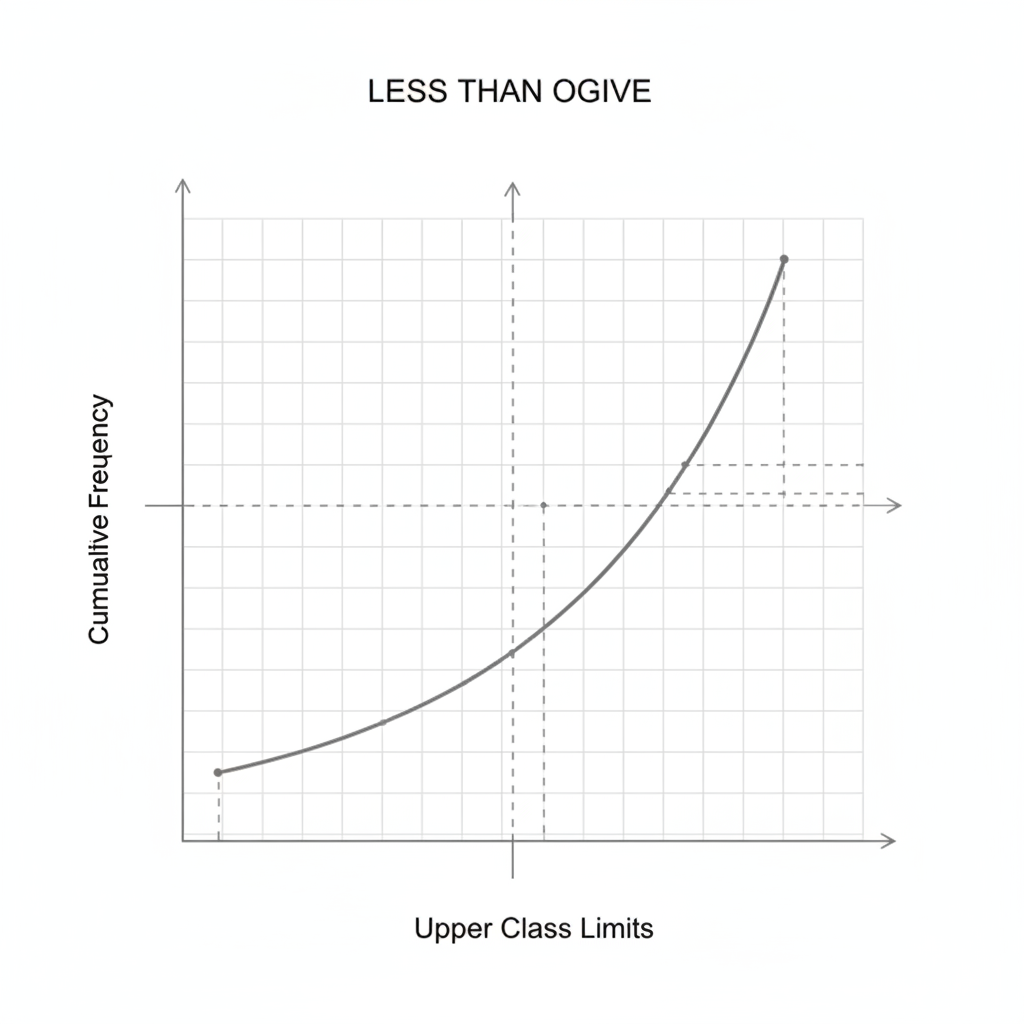 ⚠️ This picture may have spelling mistakes. Trust the words in the lesson.
What Can an Ogive Tell Us? Practical Uses!
An Ogive isn't just a pretty curve; it's a powerful tool for quickly understanding your data:
- Finding the Median: The median is the middle value of your data. On an Ogive, you can find the total cumulative frequency (e.g., 50 students). Go to half of that (25) on the y-axis, draw a horizontal line to the curve, and then drop a vertical line to the x-axis. The value on the x-axis is your median!
- Counting Above/Below a Value: Want to know how many students scored less than 75 marks? Find 75 on the x-axis, go up to the curve, then over to the y-axis. The value on the y-axis is your answer. Similarly, you can find how many scored *more* than a certain value by subtracting the 'less than' count from the total.
- Understanding Distribution: A steeper curve means data points are heavily concentrated in that region, while a flatter curve suggests data points are more spread out.
Analogy 3: A Race Progress Chart. Imagine a long-distance race. A regular graph might show you how many runners passed the 1km mark, then the 2km mark. An Ogive shows you the *total number of runners who have completed or passed* each kilometer mark. If you want to know how many runners were still in the race at the 5km mark, or how many finished *before* a certain time, the Ogive helps you visualize that running total clearly.
A Glimpse at the 'More Than' Ogive (Briefly)
While less common for introductory purposes, it's good to know that a 'More Than' Ogive exists. Instead of showing observations 'less than' an upper limit, it shows observations 'more than' a lower class limit. This curve typically starts high on the left and goes downwards to the right. But for now, mastering the 'Less Than' Ogive is your primary goal!
Conclusion: Your New Data Superpower!
Ogives might seem a little abstract at first, but with practice, you'll see how incredibly useful they are. They transform simple frequencies into a dynamic, cumulative story, allowing you to quickly answer questions about 'how many are below this point?' or 'what's the middle value?'. You've just gained a powerful tool to make sense of large datasets – go forth and explore the cumulative world of statistics!
Keep learning, free
Create a free Syllabax account to unlock practice questions and games for this topic.
Visual Learning Enhanced! 🚀
To help you master this topic, we use Advanced Syllabax AI to generate detailed diagrams and visual models.
Note on Visuals: The AI sometimes makes spelling errors in image labels. Please refer to the lesson text for the correct terminology.