Data Distribution Shapes
Watch this topic in 60 seconds
Free preview · Lesson 1
Understanding Data Distribution Shapes
Understanding Data Distribution Shapes: What's the Story Behind the Numbers?
Imagine you have a big pile of LEGO bricks. Some are small, some are large, some are red, some are blue. If you just look at the pile, it's hard to make sense of it. But what if you start sorting them? You put all the red bricks together, all the blue bricks together, and maybe even separate them by size. Suddenly, you see patterns! You notice you have way more small blue bricks than large red bricks. This process of sorting and seeing patterns is very similar to what we do when we look at data distribution shapes.
In math and statistics, 'data' is just information or numbers we collect. 'Distribution' is how that data is spread out or arranged. And 'shape' is what that arrangement looks like when we graph it. Understanding these shapes helps us tell a story about the data – what's common, what's rare, and where most of the action is happening. It's like reading the body language of numbers!
Why Do Data Shapes Matter?
Think about a class test. If most students score very high, that tells you something different than if most students score very low, or if scores are all over the place. The shape of the scores' distribution gives you a quick summary, almost like a fingerprint, of the data. It helps us:
- Understand the 'typical' value: Where do most of the numbers fall?
- Spot unusual values: Are there any extreme numbers pulling the data one way or another?
- Make predictions: What might happen next based on past patterns?
To see these shapes, we often use charts like histograms or dot plots. These charts show how many times each value (or range of values) appears in our data. The taller the bar or stack of dots, the more frequently that value occurs.
The Main Characters: Types of Distribution Shapes
1. The Bell-Shaped Star: Symmetric (Normal) Distribution
Imagine you line up all the 8th graders in your school by height. Most students would be somewhere in the middle height range, with fewer very short students and fewer very tall students. If you graph this, you'd get a shape that looks like a bell – high in the middle and sloping down equally on both sides. This is called a symmetric or normal distribution, often referred to as a bell curve.
- What it means: The data is evenly balanced around the center. If you folded the graph in half, one side would be a mirror image of the other.
- Analogy Time!
- Height of people: Most people are average height; fewer are extremely short or tall.
- Shoe sizes: Most people wear common sizes; fewer wear very small or very large sizes.
- IQ scores: The majority of people have average IQs, with fewer at the very high or very low ends.
- Weight of a bag of chips: The factory aims for a specific weight, so most bags will be very close to that weight, with a few slightly heavier or lighter.
- Key Features: In a perfect symmetric distribution, the mean (average), median (middle value), and mode (most frequent value) are all exactly the same, right at the center of the bell.
2. The 'Long Tail' to the Right: Skewed Right (Positively Skewed) Distribution
Now, let's think about something else: how much money people earn in a small town. Most people might earn a moderate amount, but then there might be a few very wealthy individuals who earn a huge amount. If you graph this, most of the data would be piled up on the left side (the lower incomes), but then there would be a long 'tail' stretching out to the right, pulled by those few very high incomes. This is a skewed right or positively skewed distribution.
- What it means: Most of the data values are concentrated on the lower end, but there are a few unusually high values (outliers) that 'pull' the distribution's tail towards the right.
- Analogy Time!
- Household income: Most families earn a moderate income, but a small number of very rich families pull the average up.
- Number of books people own: Many people own a small to moderate number of books, but avid readers or collectors might own hundreds or thousands, creating a long tail to the right.
- Waiting times at a popular restaurant: Most people wait a short time, but on very busy nights, a few might wait an extremely long time.
- Key Features: The mean (average) is usually greater than the median (middle value) because those high outliers pull the mean towards the right tail.
3. The 'Long Tail' to the Left: Skewed Left (Negatively Skewed) Distribution
What if the situation is reversed? Imagine a very easy math quiz where most students score almost perfectly (90-100%), but a few students didn't study at all and scored very low (20-30%). If you graph these scores, most of the data would be piled up on the right side (the high scores), and there would be a long 'tail' stretching out to the left, pulled by those few very low scores. This is a skewed left or negatively skewed distribution.
- What it means: Most of the data values are concentrated on the higher end, but there are a few unusually low values (outliers) that 'pull' the distribution's tail towards the left.
- Analogy Time!
- Scores on an easy test: As mentioned, most students do well, but a few struggling students create the left tail.
- Age at which people retire: Many people retire around a typical age (e.g., 60s), but some might retire much earlier due to various reasons, pulling the tail to the left.
- Lifespan of a certain brand of light bulb: Most light bulbs last a long time (manufacturers want them to!), but a small percentage might burn out much earlier.
- Key Features: The mean (average) is usually less than the median (middle value) because those low outliers pull the mean towards the left tail.
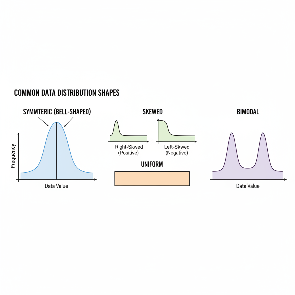
4. The Flat Landscape: Uniform Distribution
Imagine you roll a fair six-sided die many, many times. What do you expect to happen? You'd probably get roughly the same number of 1s, 2s, 3s, 4s, 5s, and 6s. If you graph this, you wouldn't see any tall peaks; instead, all the bars would be roughly the same height, forming a flat shape. This is a uniform distribution.
- What it means: All values (or categories) in the data set occur with approximately the same frequency. There are no clear peaks or valleys.
- Analogy Time!
- Rolling a fair die: Each number (1-6) has an equal chance of appearing.
- Birth month distribution: Over a very large population, the number of people born in each month tends to be roughly similar.
- Lottery numbers drawn: Each number has an equal chance of being selected, so over many drawings, their frequencies would be uniform.
- Key Features: The graph looks flat and rectangular. There isn't a single clear mode; all values are equally frequent.
5. The Double Hump: Bimodal Distribution
What if you mixed two different groups together? For example, imagine you measured the heights of a group of adult men and a group of adult women. Men tend to be taller than women on average. So, if you plotted all their heights together, you'd likely see two distinct peaks: one peak for the average height of women and another peak for the average height of men. This is called a bimodal distribution (bi- means two).
- What it means: The data has two distinct peaks, indicating that there are two different clusters or groups within the data. This often suggests that two different populations or processes are being measured together.
- Analogy Time!
- Test scores from two different classes: If one class found a test very easy and another found it very hard, you might see a peak of high scores and a peak of low scores.
- Customer satisfaction ratings for a new product: If some customers love it and others hate it, you might see peaks at 'very satisfied' and 'very dissatisfied'.
- Traffic patterns: The number of cars on the road during rush hour might show two peaks – one in the morning and one in the evening.
- Key Features: The graph shows two distinct modes (two highest points). The mean and median might fall between these two peaks or closer to one, depending on the number of data points in each group.
Putting It All Together: The Story of Your Data
Understanding data distribution shapes is a fundamental skill. It helps you quickly grasp the main characteristics of a dataset without having to look at every single number. Just like knowing if a story is a comedy, a tragedy, or a mystery changes how you understand it, knowing the shape of your data helps you interpret its meaning and draw better conclusions. Whether you're looking at test scores, economic data, or scientific measurements, these shapes are the secret language of numbers, waiting for you to decipher them!
Keep learning, free
Create a free Syllabax account to unlock practice questions and games for this topic.
Visual Learning Enhanced! 🚀
To help you master this topic, we use Advanced Syllabax AI to generate detailed diagrams and visual models.
Note on Visuals: The AI sometimes makes spelling errors in image labels. Please refer to the lesson text for the correct terminology.