Introduction to Histograms
Watch this topic in 60 seconds
Free preview · Lesson 1
Understanding Introduction to Histograms
Introduction to Histograms: Unlocking Data Stories (Grade 7)
What's a Histogram and Why Do We Need Them?
Imagine you have a huge pile of numbers – maybe the heights of all students in your school, or the scores from a big math test. How do you make sense of it all? Just looking at a long list of numbers can be confusing! This is where histograms come to the rescue!
A histogram is a special type of graph that helps us understand and visualize large amounts of numerical data. It shows us how often different values or ranges of values appear in a dataset. Think of it as a storyteller for numbers, showing you the overall picture instead of individual tiny details.
Analogy 1: The Cookie Cutter Machine!
Imagine you have a big blob of cookie dough (your raw data). If you just cut out one cookie at a time, you'd have hundreds of individual cookies (individual data points). That's a lot to look at! Instead, a histogram is like a special cookie cutter machine that groups similar-sized cookies together into different trays. One tray might hold all cookies between 2 and 3 inches, another for 3 to 4 inches, and so on. The number of cookies in each tray tells you how common that size is!
Categorical vs. Continuous Data: The Big Difference!
Before we dive deeper, it's important to understand two types of data:
- Categorical Data: This is data that can be put into groups or categories. Think of your favorite colors (red, blue, green), types of pets (dog, cat, fish), or favorite sports (soccer, basketball, tennis). You count how many are in each category. For this, we often use bar graphs.
- Continuous Data: This is data that can take any value within a certain range. It's usually measured, not counted in distinct categories. Examples include heights (you can be 150 cm, 150.5 cm, 150.57 cm!), weights, temperatures, time, or test scores. There are usually too many possible exact values to list them all individually. This is where histograms shine!
Analogy 2: Sorting Your Toys!
If you're sorting toys by type (Lego, action figures, stuffed animals), that's like categorical data – you'd use a bar graph. But if you're sorting your Lego bricks by their weight or length, that's continuous data. You wouldn't have a bin for '1.234 grams' and another for '1.235 grams' – you'd group them: '0-5 grams', '6-10 grams', etc. This grouping is key for continuous data!
Frequency and Bins (or Intervals): The Histogram's Building Blocks
1. Frequency: How Often Does It Happen?
Frequency simply means how many times something occurs. If 10 students scored between 80 and 89 on a test, then the frequency for that score range is 10.
2. Bins or Intervals: Grouping the Data
Since continuous data has so many possible values, we can't make a bar for every single one. Instead, we group the data into ranges. These ranges are called bins or intervals. Each bin covers a specific range of values, and all bins are usually the same width.
Analogy 3: Sorting Laundry!
Imagine you have a mountain of socks, and you want to sort them by size. You wouldn't make a pile for size '5', another for '5.1', another for '5.2', and so on. That would be impossible! Instead, you make bigger piles (your 'bins'): 'Small' (sizes 4-6), 'Medium' (sizes 7-9), 'Large' (sizes 10-12). Each pile represents an interval, and the number of socks in each pile is its frequency.
The Anatomy of a Histogram: What You See
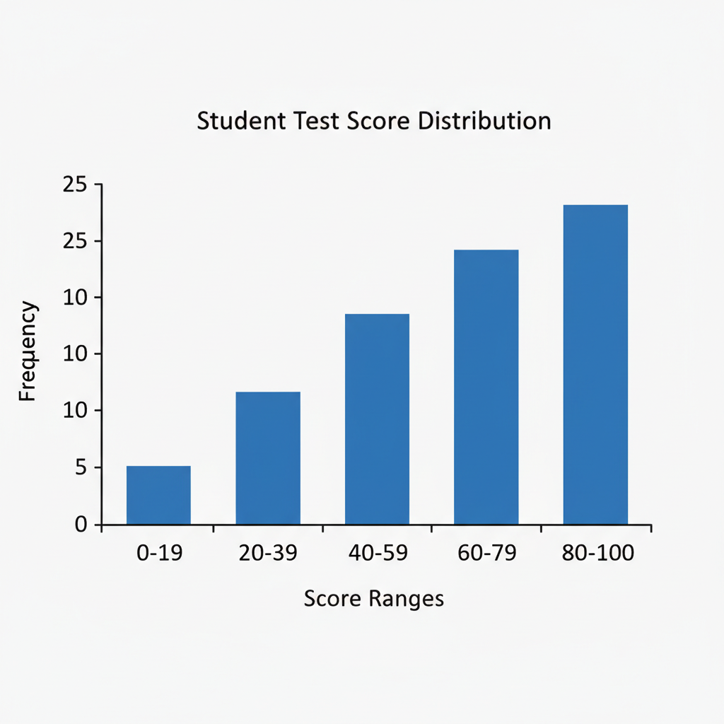
A histogram looks a lot like a bar graph, but with a few crucial differences:
-
X-axis (Horizontal Axis): The Data Intervals
This axis shows the numerical ranges (our 'bins' or 'intervals') of your continuous data. For example, if you're looking at test scores, the X-axis might show '50-59', '60-69', '70-79', and so on.
-
Y-axis (Vertical Axis): The Frequency
This axis tells you 'how many' or 'how often' data points fall into each interval. It's the count of items within each bin.
-
The Bars: Touching Rectangles!
Each bar represents a specific interval, and its height shows the frequency for that interval. The most important visual difference from a regular bar graph is that the bars in a histogram always touch each other. Why? Because the data is continuous, meaning there are no gaps between the intervals on the X-axis. For example, if one bin ends at 69 and the next starts at 70, there's no 'missing' score between 69 and 70 (in many cases, 69.9 would be rounded up or down, or there's a convention for including boundaries).
Analogy 4: The City Skyline!
Imagine looking at a city skyline. Each building is like a 'bin' (a range of building heights, for example). The height of each building tells you how many buildings fall into that height range (its frequency). The buildings stand right next to each other because there's a continuous range of possible building heights in a city – there are no 'empty spaces' between height ranges.
Histogram vs. Bar Graph: The Key Differences Summarized
While they look similar, remember these key distinctions:
- Data Type: Histograms are for continuous numerical data (like heights, weights, ages). Bar graphs are for categorical data (like types of pets, favorite colors).
- Bars: In histograms, the bars touch each other. In bar graphs, the bars usually have gaps between them.
- X-axis: In histograms, the X-axis shows ranges of numbers (intervals). In bar graphs, the X-axis shows separate categories.
Why Are Histograms So Useful?
Histograms help us quickly see important features of our data:
- Shape of the Data: Is it symmetrical? Skewed (more data on one side)?
- Central Tendency: Where do most of the values fall? Are they clustered in the middle, or towards the beginning or end?
- Spread of the Data: Are the values tightly packed together or spread out widely?
- Outliers: Are there any unusually high or low values that stand far apart from the others?
By looking at a histogram, you can tell if most students got high scores, low scores, or if the scores were pretty evenly spread out. It's a powerful tool for understanding the 'story' behind your numbers!
Let's Summarize!
Histograms are like super-powered bar graphs designed for continuous numbers. They help us group vast amounts of information into manageable 'bins' and visually show us how often certain things happen. They are essential tools for anyone wanting to understand patterns and trends in data, from scientists and economists to everyday students making sense of their test scores!
Keep learning, free
Create a free Syllabax account to unlock practice questions and games for this topic.
Visual Learning Enhanced! 🚀
To help you master this topic, we use Advanced Syllabax AI to generate detailed diagrams and visual models.
Note on Visuals: The AI sometimes makes spelling errors in image labels. Please refer to the lesson text for the correct terminology.