Measures of Spread: Quartiles
Watch this topic in 60 seconds
Free preview · Lesson 1
Understanding Measures of Spread: Quartiles
Measures of Spread: Quartiles (Grade 9, Foundational)
Welcome, future data detectives! Today, we're going to embark on an exciting journey to understand 'Measures of Spread,' specifically focusing on something called Quartiles. Think of data as a story – we often want to know more than just the main character (the average). We want to know how the story unfolds, how spread out the events are, or how varied the characters are!
Why Do We Care About Spread?
Imagine two groups of students taking a math test. Both groups have an average score of 70%. Does this mean they performed exactly the same? Not necessarily! In one group, everyone might have scored between 65% and 75%. In the other, half might have scored 20% and the other half 120% (if extra credit was given!). While both average to 70%, the spread of scores is vastly different. Measures of spread tell us how diverse or consistent our data is. It's like knowing not just the average height of students in a class, but also if everyone is roughly the same height, or if there's a huge difference between the shortest and tallest.
Introducing Quartiles: Dividing Your Data Pizza!
Think of your entire set of ordered data as a delicious, rectangular pizza. When you want to share that pizza fairly, what's the first thing you do? You cut it in half! Then, you might cut each of those halves in half again. Voila! You now have four equal slices. This is exactly what quartiles do to your data set!
Quartiles (pronounced KWAR-tiles) are values that divide a dataset into four equal parts, or quarters, after the data has been arranged in order from smallest to largest. Each part contains 25% of the data points. They help us understand the distribution of the data without just relying on the average.
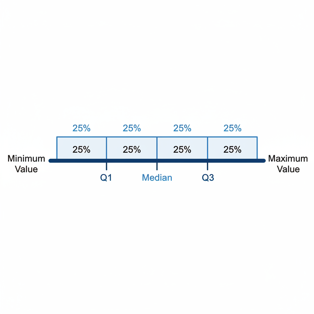
Let's Meet the Quartile Family:
- The Median (Q2 - Second Quartile): This is the 'middle child' of our data family. It's the value that cuts your entire ordered dataset exactly in half. 50% of the data points are below the median, and 50% are above it. We've learned about the median before – it's crucial for finding the other quartiles!
- Q1 (First Quartile): This is like the 'youngest child' among the dividing points. Q1 is the median of the lower half of your data. This means 25% of your data points are below Q1, and 75% are above it.
- Q3 (Third Quartile): This is like the 'oldest child' among the dividing points. Q3 is the median of the upper half of your data. This means 75% of your data points are below Q3, and only 25% are above it.
So, we have Q1, Q2 (Median), and Q3. These three values divide your data into four sections, each containing 25% of the observations.
How to Find Quartiles: A Step-by-Step Guide!
Finding quartiles is like following a simple recipe. Let's try it with an example!
Example Data Set: The number of points scored by a basketball player in 9 games: 12, 18, 9, 21, 15, 10, 25, 14, 16
Step 1: Arrange the Data in Order
This is super important! Quartiles only make sense when your data is ordered from smallest to largest.
Ordered Data: 9, 10, 12, 14, 15, 16, 18, 21, 25
Step 2: Find the Median (Q2)
The median is the middle value. If you have an odd number of data points, it's the exact middle one. If you have an even number, it's the average of the two middle values.
Our data set has 9 points. The middle value is the 5th value:
9, 10, 12, 14, 15, 16, 18, 21, 25
Q2 (Median) = 15
Step 3: Find Q1 (First Quartile)
Now, we look at the 'lower half' of the data. This includes all the numbers BEFORE the median (Q2).
Lower Half: 9, 10, 12, 14
We need to find the median of this lower half. Since there are 4 numbers (an even amount), we take the average of the two middle numbers.
The two middle numbers are 10 and 12.
(10 + 12) / 2 = 22 / 2 = 11
Q1 = 11
Step 4: Find Q3 (Third Quartile)
Next, we look at the 'upper half' of the data. This includes all the numbers AFTER the median (Q2).
Upper Half: 16, 18, 21, 25
Now, find the median of this upper half. Again, 4 numbers, so average the two middle ones.
The two middle numbers are 18 and 21.
(18 + 21) / 2 = 39 / 2 = 19.5
Q3 = 19.5
So, for our basketball player's scores, the quartiles are:
- Q1 = 11
- Q2 (Median) = 15
- Q3 = 19.5
This tells us that 25% of the time, the player scored 11 points or less. 50% of the time, they scored 15 points or less. And 75% of the time, they scored 19.5 points or less.
Interquartile Range (IQR): The Middle Ground!
Once you have Q1 and Q3, you can easily calculate something called the Interquartile Range (IQR). The IQR is simply the difference between Q3 and Q1 (IQR = Q3 - Q1).
Think of it like this: if Q1 marks the point where the bottom 25% of data ends, and Q3 marks the point where the top 25% of data begins, then the space *between* Q1 and Q3 contains the middle 50% of your data. The IQR tells you how spread out that middle 50% is.
For our basketball player's scores:
IQR = Q3 - Q1 = 19.5 - 11 = 8.5
A smaller IQR means the middle 50% of your data points are clustered closer together (less spread), while a larger IQR means they are more spread out.
In Summary: Why Quartiles Matter
Quartiles give us a much richer understanding of our data than just the mean or median alone. They show us how the data is distributed, allowing us to identify where the bulk of the values lie, and spot any unusual values (outliers) that might be far from the middle. They are powerful tools in statistics, helping us make better sense of the numbers all around us!
Keep learning, free
Create a free Syllabax account to unlock practice questions and games for this topic.
Visual Learning Enhanced! 🚀
To help you master this topic, we use Advanced Syllabax AI to generate detailed diagrams and visual models.
Note on Visuals: The AI sometimes makes spelling errors in image labels. Please refer to the lesson text for the correct terminology.